T-test on real data using tidyverse
Introduction
A t-test is a statistical test used to compare means between groups or against a known value. This tutorial demonstrates how to perform t-tests using tidyverse tools for data manipulation and analysis, making the process more intuitive and reproducible.
Getting Started
library(tidyverse)
library(palmerpenguins)
Example 1: One-Sample T-test
The Problem
We want to test whether the average body mass of penguins differs significantly from a hypothesized population mean of 4000 grams.
Step 1: Explore the Data
Let’s examine the penguin body mass data to understand its distribution.
penguins |>
  select(body_mass_g) |>
  drop_na() |>
  summary()
This shows us the basic statistics for penguin body mass, including the mean and quartiles.
Step 2: Visualize the Distribution
Creating a histogram helps us assess normality before running the t-test.
penguins |>
  drop_na(body_mass_g) |>
  ggplot(aes(x = body_mass_g)) +
  geom_histogram(bins = 20, alpha = 0.8, fill = "steelblue", color = "white") +
  geom_vline(xintercept = 4000, color = "red", linetype = "dashed",
             linewidth = 1.2) +
  labs(title = "Distribution of Penguin Body Mass",
       subtitle = "Red dashed line: hypothesized population mean (4000g) for one-sample t-test",
       x = "Body Mass (g)", y = "Count") +
  theme_minimal()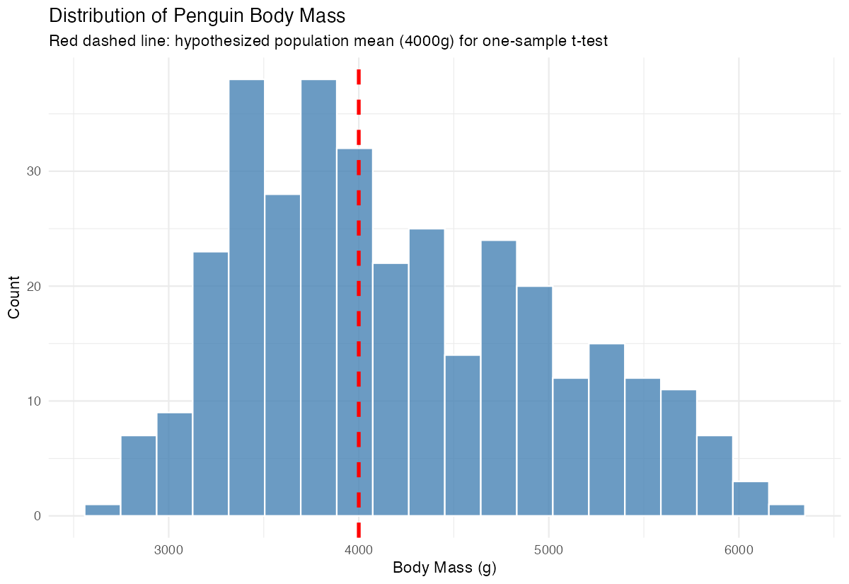
The histogram shows the distribution of body mass with our hypothesized mean marked in red.
Step 3: Perform One-Sample T-test
Now we test if the mean body mass significantly differs from 4000 grams.
penguin_mass <- penguins |>
  drop_na(body_mass_g) |>
  pull(body_mass_g)

t.test(penguin_mass, mu = 4000)
The t-test results show a significant difference (p < 0.05), indicating penguin body mass differs from 4000 grams.
Example 2: Two-Sample T-test
The Problem
We want to compare body mass between male and female penguins to determine if there’s a significant difference between sexes. This is a common research question in biological studies.
Step 1: Prepare the Data
First, we’ll clean the data and examine the sample sizes for each group.
penguin_sex_data <- penguins |>
  filter(!is.na(body_mass_g), !is.na(sex)) |>
  select(sex, body_mass_g)

penguin_sex_data |>
  count(sex)
This gives us clean data with body mass and sex information, showing balanced sample sizes.
Step 2: Compare Group Means
Let’s calculate summary statistics for each group to preview potential differences.
penguin_sex_data |>
  group_by(sex) |>
  summarise(
    mean_mass = mean(body_mass_g),
    sd_mass = sd(body_mass_g),
    n = n()
  )
The summary shows clear differences in average body mass between male and female penguins.
Step 3: Visualize Group Differences
A boxplot effectively shows the distribution differences between groups.
penguin_sex_data |>
  ggplot(aes(x = sex, y = body_mass_g, fill = sex)) +
  geom_boxplot(alpha = 0.7, outlier.shape = NA) +
  geom_jitter(width = 0.15, alpha = 0.5) +
  labs(title = "Penguin Body Mass by Sex",
       subtitle = "Two-sample t-test comparison of body mass between sexes",
       x = "Sex", y = "Body Mass (g)") +
  theme_minimal() +
  theme(legend.position = "none")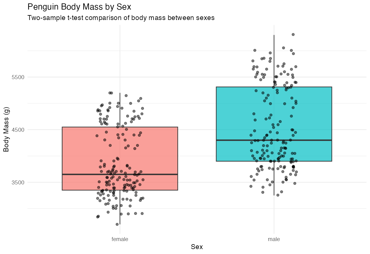
The boxplot reveals that male penguins appear to have higher body mass than females.
Step 4: Perform Two-Sample T-test
Now we’ll test if the observed difference is statistically significant.
male_mass <- penguin_sex_data |>
  filter(sex == "male") |>
  pull(body_mass_g)

female_mass <- penguin_sex_data |>
  filter(sex == "female") |>
  pull(body_mass_g)

t.test(male_mass, female_mass)
The t-test confirms a highly significant difference (p < 0.001) in body mass between male and female penguins.
Step 5: Alternative Approach Using Formula
We can also perform the same test using R’s formula interface for cleaner code.
t.test(body_mass_g ~ sex, data = penguin_sex_data)This produces identical results but with more concise syntax using the formula notation.
Summary
- One-sample t-tests compare a sample mean against a hypothesized population value
- Two-sample t-tests compare means between two independent groups
- Always visualize your data before testing to check assumptions and understand distributions
- Clean your data by removing missing values before analysis using
drop_na() The tidyverse approach makes data preparation and exploration more intuitive and reproducible