How to use geom_raster() in R

Learn how to use geom_raster() in R with practical examples. Step-by-step guide with code you can copy and run immediately.

Introduction

geom_raster() is a ggplot2 function that creates rectangular tiles to visualize data on a grid, similar to a heatmap. It’s particularly useful for displaying matrix-like data, spatial information, or any dataset where you want to show relationships between two continuous variables using color intensity.

Getting Started

library(tidyverse)
library(palmerpenguins)

Example 1: Basic Usage

The Problem

We want to create a simple heatmap showing the relationship between two variables using rectangular tiles. Let’s visualize how penguin bill length varies across different body mass ranges.

Step 1: Prepare the Data

First, we’ll create bins for our continuous variables to form a grid.

penguin_grid <- penguins |>
  filter(!is.na(bill_length_mm), !is.na(body_mass_g)) |>
  mutate(
    mass_bin = cut(body_mass_g, breaks = 8),
    bill_bin = cut(bill_length_mm, breaks = 6)
  )

This creates categorical bins from our continuous variables for the raster grid.

Step 2: Calculate Summary Statistics

Now we’ll count penguins in each grid cell to create our fill values.

raster_data <- penguin_grid |>
  group_by(mass_bin, bill_bin) |>
  summarise(count = n(), .groups = 'drop') |>
  filter(!is.na(mass_bin), !is.na(bill_bin))

Each combination of mass and bill length bins now has a count value for coloring.

Step 3: Create Basic Raster Plot

Let’s create our first raster visualization.

ggplot(raster_data, aes(x = mass_bin, y = bill_bin, fill = count)) +
  geom_raster() +
  scale_fill_gradient(low = "white", high = "darkblue") +
  labs(title = "Penguin Counts by Body Mass and Bill Length Bins",
       x = "Body Mass Bin", y = "Bill Length Bin", fill = "Count") +
  theme_minimal() +
  theme(axis.text.x = element_text(angle = 45, hjust = 1))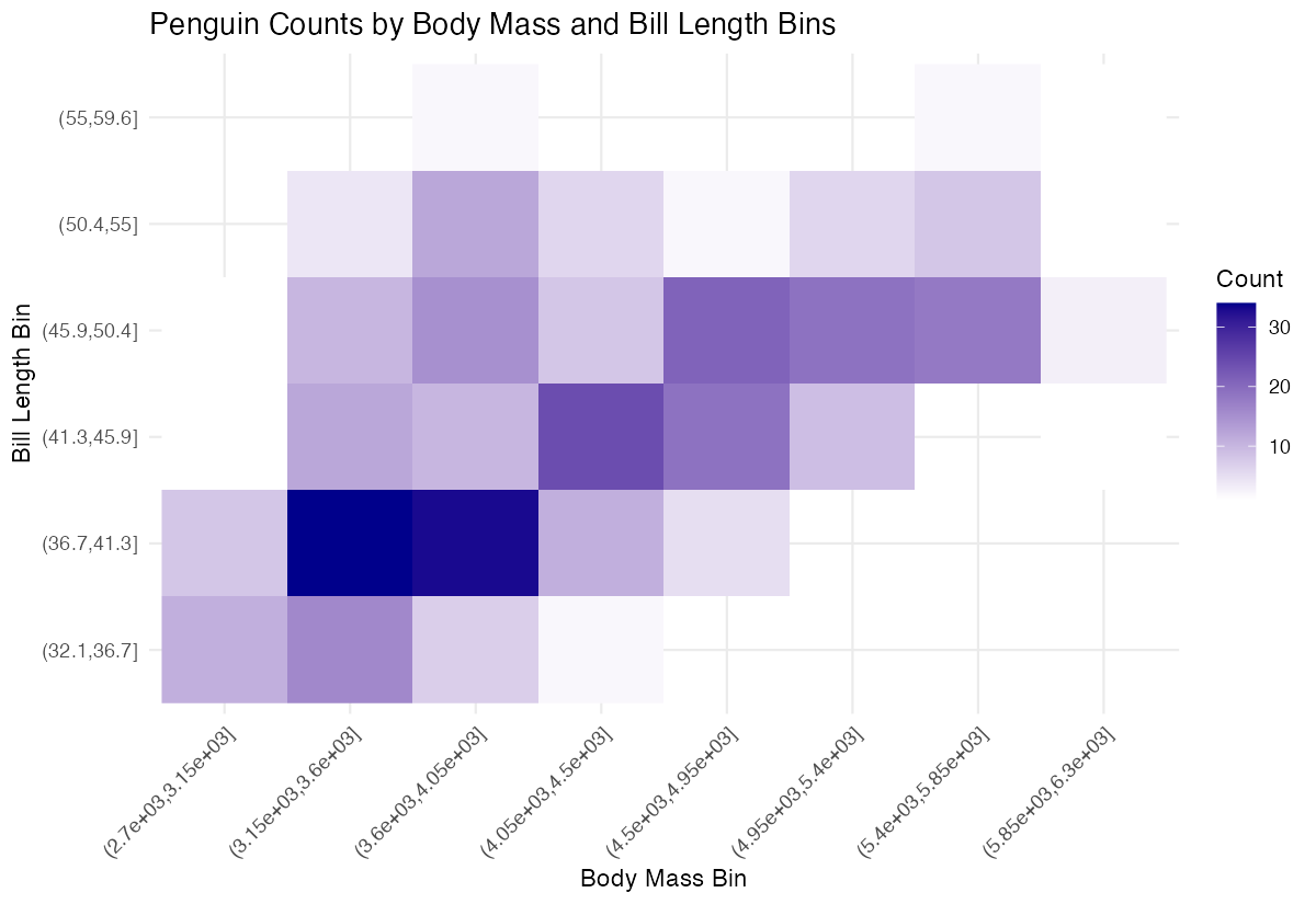

Raster heatmap in R using geom_raster() in ggplot2 showing penguin counts across binned body mass and bill length with blue gradient

This produces a basic heatmap where darker colors represent higher penguin counts in each grid cell.

Example 2: Practical Application

The Problem

We want to create a more sophisticated analysis showing the average flipper length across different combinations of bill length and body mass. This helps identify patterns in penguin morphology that might indicate different species clusters.

Step 1: Create Analysis Dataset

We’ll prepare data with more refined bins and calculate average flipper length.

morphology_data <- penguins |>
  filter(!is.na(bill_length_mm), !is.na(body_mass_g), !is.na(flipper_length_mm)) |>
  mutate(
    mass_group = round(body_mass_g / 200) * 200,
    bill_group = round(bill_length_mm / 2) * 2
  )

This creates evenly spaced groups for body mass (200g intervals) and bill length (2mm intervals).

Step 2: Calculate Flipper Averages

Now we’ll compute the mean flipper length for each combination.

flipper_summary <- morphology_data |>
  group_by(mass_group, bill_group) |>
  summarise(
    avg_flipper = mean(flipper_length_mm),
    n_penguins = n(),
    .groups = 'drop'
  ) |>
  filter(n_penguins >= 3)

We filter to keep only combinations with at least 3 penguins for reliable averages.

Step 3: Create Enhanced Visualization

Let’s build a polished raster plot with better styling and labels.

ggplot(flipper_summary, aes(x = mass_group, y = bill_group, fill = avg_flipper)) +
  geom_raster() +
  scale_fill_viridis_c(name = "Average\nFlipper\nLength (mm)") +
  labs(
    title = "Penguin Flipper Length by Body Mass and Bill Length",
    x = "Body Mass (g)",
    y = "Bill Length (mm)"
  )

This creates a professional-looking heatmap using the viridis color scale for better accessibility.

Step 4: Add Final Touches

We’ll enhance the plot with better formatting and theme adjustments.

ggplot(flipper_summary, aes(x = mass_group, y = bill_group, fill = avg_flipper)) +
  geom_raster() +
  scale_fill_viridis_c(name = "Flipper\nLength\n(mm)") +
  labs(
    title = "Penguin Flipper Length by Body Mass and Bill Length",
    x = "Body Mass (g)",
    y = "Bill Length (mm)"
  ) +
  theme_minimal() +
  theme(
    axis.text.x = element_text(angle = 45, hjust = 1),
    plot.title = element_text(hjust = 0.5)
  )

Viridis raster plot in R using geom_raster() showing average penguin flipper length across body mass and bill length groups in ggplot2

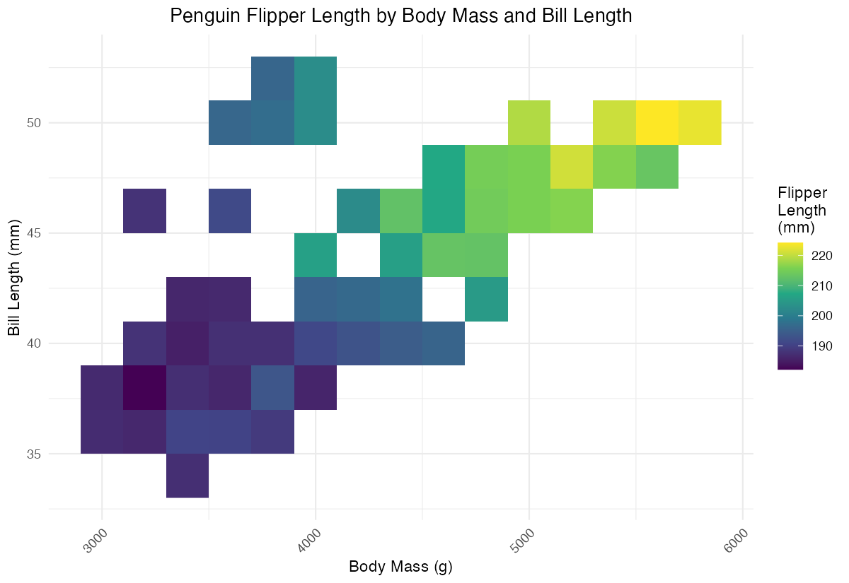
The final plot clearly shows morphological patterns, with distinct clusters likely representing different penguin species.

Summary

• geom_raster() creates rectangular tiles perfect for heatmap-style visualizations of gridded data
• Always ensure your data has x, y, and fill aesthetics defined before using this geom
• Use scale_fill_gradient() or scale_fill_viridis_c() to customize color schemes for continuous data
• Bin continuous variables appropriately to create meaningful grid cells for analysis

• Combine with theme_minimal() and custom themes for professional-looking scientific visualizations

Related Posts

• How to use geom_point() in R
• How to use geom_area() in R
• How to use geom_tile() in R
• How to use select() in R
• How to use mutate() in R