How to use scale_color_manual() in R
Introduction
The scale_color_manual() function in ggplot2 allows you to manually specify colors for different groups in your plots. This gives you complete control over your color scheme, making it perfect when you need specific brand colors, want to ensure accessibility, or simply prefer custom aesthetics over ggplot2’s default color palette.
Getting Started
library(tidyverse)
library(palmerpenguins)
Example 1: Basic Usage
The Problem
By default, ggplot2 automatically assigns colors to different groups in your data. However, these default colors might not match your preferences or requirements for a professional presentation.
Step 1: Create a basic plot with default colors
First, let’s create a scatter plot to see ggplot2’s default color scheme.
basic_plot <- penguins |>
  ggplot(aes(x = bill_length_mm, y = bill_depth_mm,
             color = species)) +
  geom_point(size = 3)

basic_plot
This creates a scatter plot where each penguin species gets a different default color automatically.
Step 2: Apply custom colors manually
Now we’ll override the default colors with our own choices using scale_color_manual().
custom_plot <- penguins |>
  ggplot(aes(x = bill_length_mm, y = bill_depth_mm,
             color = species)) +
  geom_point(size = 3) +
  scale_color_manual(values = c("red", "blue", "green"))

custom_plot
The plot now uses our specified colors: red, blue, and green for the three penguin species.
Step 3: Use better color choices
Let’s improve our color selection with more professional hex codes.
professional_plot <- penguins |>
ggplot(aes(x = bill_length_mm, y = bill_depth_mm,
color = species)) +
geom_point(size = 3) +
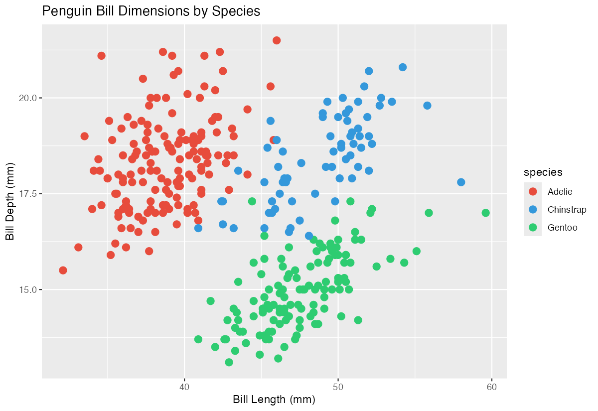
scale_color_manual(values = c("#E74C3C", "#3498DB", "#2ECC71"))
professional_plotThese hex codes provide more sophisticated colors that work well together and maintain good contrast.
Example 2: Practical Application
The Problem
You’re creating a report for stakeholders about car performance data, and you need the colors to match your company’s brand guidelines. Additionally, you want to ensure the legend shows meaningful labels rather than the raw data values.
Step 1: Examine the data structure
Let’s look at our car data and create a basic plot to understand what we’re working with.
mtcars |>
  ggplot(aes(x = wt, y = mpg, color = factor(cyl))) +
  geom_point(size = 4) +
  labs(x = "Weight (1000 lbs)", y = "Miles per Gallon")
This shows the relationship between car weight and fuel efficiency, colored by number of cylinders.
Step 2: Apply brand colors with custom labels
Now we’ll apply specific brand colors and improve the legend labels for better presentation.
branded_plot <- mtcars |>
  ggplot(aes(x = wt, y = mpg, color = factor(cyl))) +
  geom_point(size = 4) +
  scale_color_manual(
    values = c("4" = "#1f4e79", "6" = "#70ad47", "8" = "#c55a5a"),
    labels = c("4 Cylinder", "6 Cylinder", "8 Cylinder"),
    name = "Engine Type"
  )

branded_plot
The plot now uses brand-specific colors and displays professional labels in the legend.
Step 3: Add finishing touches
Let’s complete the visualization with proper titles and theme adjustments.
final_plot <- mtcars |>
ggplot(aes(x = wt, y = mpg, color = factor(cyl))) +
geom_point(size = 4) +
scale_color_manual(
values = c("4" = "#1f4e79", "6" = "#70ad47", "8" = "#c55a5a"),
labels = c("4 Cylinder", "6 Cylinder", "8 Cylinder"),
name = "Engine Type"
) +
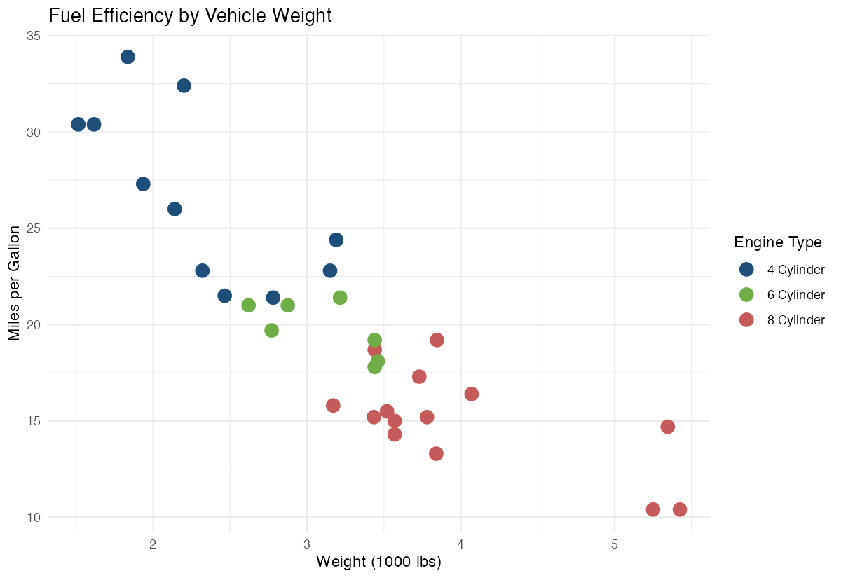
labs(title = "Fuel Efficiency by Vehicle Weight",
x = "Weight (1000 lbs)", y = "Miles per Gallon") +
theme_minimal()
final_plotThe final visualization is now publication-ready with custom colors, clear labels, and professional styling.
Summary
scale_color_manual()gives you complete control over color choices in ggplot2 visualizations- Use the
valuesparameter to specify colors either by name (“red”) or hex codes (“#E74C3C”) - The
labelsparameter lets you customize legend text for better readability - The
nameparameter changes the legend title to something more descriptive Combine with other ggplot2 elements like
labs()andtheme_minimal()for professional-looking plots