How to Perform a Chi-Square Test in R
Introduction
The chi-square test is a statistical method used to determine whether there’s a significant association between two categorical variables. It’s commonly used to test independence between variables or to compare observed frequencies with expected frequencies in your data.
When to use a chi-square test: - Testing if two categorical variables are independent - Comparing observed frequencies to expected frequencies - Analyzing survey data with categorical responses - Testing goodness of fit to a theoretical distribution
The Math Behind Chi-Square
The chi-square statistic measures how much observed frequencies differ from expected frequencies:
χ² = Σ [(Observed - Expected)² / Expected]For each cell in the contingency table: 1. Calculate the expected frequency: Expected = (Row Total × Column Total) / Grand Total 2. Compute (Observed - Expected)² / Expected 3. Sum across all cells
Degrees of freedom = (rows - 1) × (columns - 1)
The larger the χ² value, the stronger the evidence against independence. The p-value tells you the probability of seeing such a large χ² if the variables were truly independent.
Getting Started
library(tidyverse)
library(palmerpenguins)
Example 1: Basic Usage
The Problem
We want to test whether there’s an association between penguin species and the island they live on. This will help us understand if certain species prefer specific islands.
Step 1: Prepare the Data
First, we’ll examine our data and create a contingency table.
# Load and inspect the penguins data
data(penguins)
penguins_clean <- penguins |>
  filter(!is.na(species), !is.na(island))

head(penguins_clean)
This creates a clean dataset without missing values for our variables of interest.
Step 2: Create Contingency Table
We need to organize our data into a cross-tabulation format.
# Create contingency table
penguin_table <- table(penguins_clean$species,
                      penguins_clean$island)
penguin_table
The table shows the count of each species on each island, which forms the basis for our chi-square test.
Step 3: Perform Chi-square Test
Now we’ll conduct the actual statistical test.
# Perform chi-square test
chi_result <- chisq.test(penguin_table)
chi_result
The test returns a chi-square statistic, degrees of freedom, and p-value to determine statistical significance.
Step 4: Interpret Results
Let’s examine the expected frequencies and residuals.
# View expected frequencies
chi_result$expected

# View standardized residuals
chi_result$stdres
Expected frequencies show what we’d expect if there was no association, while residuals indicate which combinations contribute most to the chi-square statistic.
Example 2: Practical Application
The Problem
A researcher wants to determine if there’s a relationship between car transmission type (automatic vs manual) and number of cylinders in the mtcars dataset. This could inform decisions about car manufacturing and consumer preferences.
Step 1: Prepare the Data
We’ll convert the transmission variable and create cylinder categories.
# Prepare mtcars data
cars_data <- mtcars |>
  mutate(transmission = ifelse(am == 0, "Automatic", "Manual"),
         cyl_group = as.factor(cyl))

head(cars_data[c("transmission", "cyl_group")])
This creates clear categorical variables for our analysis with meaningful labels.
Step 2: Create and Examine Contingency Table
Let’s build our cross-tabulation and visualize the relationship.
# Create contingency table
car_table <- table(cars_data$transmission,
                  cars_data$cyl_group)
car_table
The table reveals the distribution of transmission types across different cylinder counts.
Step 3: Perform Chi-square Test with Assumptions Check
We’ll test our hypothesis while checking if assumptions are met.
# Check if expected frequencies are adequate
chi_test <- chisq.test(car_table)
chi_test$expected

# Perform the test
chi_test
All expected frequencies should be at least 5 for the chi-square test to be valid.
Step 4: Calculate Effect Size
We’ll compute Cramér’s V to measure the strength of association.
# Calculate Cramér's V
cramers_v <- sqrt(chi_test$statistic /
                 (sum(car_table) * (min(dim(car_table)) - 1)))
cramers_v
Cramér’s V ranges from 0 to 1, where higher values indicate stronger associations between variables.
Step 5: Visualize the Results
Create a visualization to better understand the relationship.
# Create a visualization
car_df <- as.data.frame(car_table)
names(car_df) <- c("Transmission", "Cylinders", "Count")

ggplot(car_df, aes(x = Cylinders, y = Count, fill = Transmission)) +
  geom_col(position = "dodge", alpha = 0.9) +
  labs(title = "Transmission Type vs Cylinder Count",
       x = "Number of Cylinders", y = "Count") +
  theme_minimal()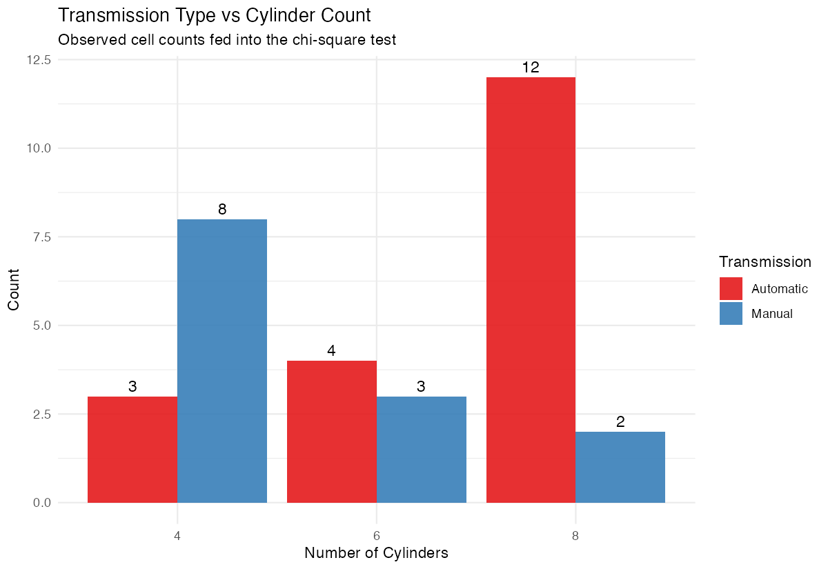
The bar chart provides a visual representation of the association we’re testing statistically.
Assumptions and Limitations
Key assumptions of the chi-square test:
- Random sampling: Data should come from a random sample
- Independence: Each observation should be independent
- Expected frequency rule: At least 80% of cells should have expected frequency ≥ 5
- Mutually exclusive categories: Each observation belongs to exactly one cell
Check the expected frequency assumption:
# View expected frequencies
chi_result$expected

# Count cells with expected frequency < 5
sum(chi_result$expected < 5)
When assumptions are violated:
# Use Fisher's exact test for small samples
fisher.test(penguin_table)

# Use Monte Carlo simulation for larger tables with small expected frequencies
chisq.test(penguin_table, simulate.p.value = TRUE, B = 10000)
Don’t use chi-square when: - Expected frequencies are too small (use Fisher’s exact test) - Data are paired or matched (use McNemar’s test) - You have ordinal categories and want to test for trend (use Cochran-Armitage test)
Common Mistakes
1. Using percentages instead of counts
# Wrong - using proportions
wrong_table <- prop.table(penguin_table)
chisq.test(wrong_table)  # Incorrect!

# Correct - use raw counts
chisq.test(penguin_table)
2. Ignoring the expected frequency warning
R will warn you when expected frequencies are too small, but it still runs the test. Always check chi_result$expected and consider Fisher’s exact test if many cells are < 5.
3. Confusing significance with effect size
A significant p-value doesn’t mean a strong association. Always report effect size:
# Cramér's V for effect size
# Small: 0.1, Medium: 0.3, Large: 0.5
cramers_v <- sqrt(chi_result$statistic /
                 (sum(penguin_table) * (min(dim(penguin_table)) - 1)))
4. Testing the wrong hypothesis
Chi-square tests association, not causation or direction. It tells you variables are related, not how they’re related. Examine the contingency table and residuals to understand the nature of the association.
Summary
- Chi-square tests determine independence between two categorical variables using observed vs expected frequencies
- Always check that expected frequencies are ≥5 in each cell before interpreting results
- P-values < 0.05 suggest a significant association between variables exists
- Examine standardized residuals to identify which combinations drive significant results
- Calculate Cramér’s V for effect size when you find significant associations