How to one-sample t-test in R
Introduction
The one-sample t-test is a statistical hypothesis test used to determine whether a sample mean significantly differs from a known population mean. Unlike the z-test, which requires knowing the population standard deviation, the t-test uses the sample standard deviation, making it much more practical for real-world applications.
You would use a one-sample t-test when you have a single sample and want to compare its mean to a theoretical value, industry standard, or historical benchmark. Common scenarios include testing whether a new manufacturing process produces items with a target weight, checking if students’ test scores differ from a national average, or verifying if a medication achieves its intended effect.
The one-sample t-test requires several assumptions: the data should be approximately normally distributed (especially important for small samples), observations must be independent of each other, and the data should be measured at the interval or ratio level. The test is relatively robust to minor violations of normality, particularly with larger sample sizes (n > 30), thanks to the Central Limit Theorem.
The Math
The one-sample t-test uses this formula:
t = (sample_mean - population_mean) / (sample_standard_deviation / sqrt(sample_size))Breaking this down: - t: the t-statistic we calculate - sample_mean: the average of your observed data - population_mean: the value you’re testing against (your null hypothesis) - sample_standard_deviation: the standard deviation of your sample - sample_size: the number of observations in your sample
The denominator (sample_standard_deviation / sqrt(sample_size)) is called the standard error of the mean. The t-statistic follows a t-distribution with (n-1) degrees of freedom, where n is your sample size.
R Implementation
Let’s start by loading the necessary packages and exploring our data:
library(tidyverse)
library(palmerpenguins)

# Look at the penguins dataset
glimpse(penguins)
Rows: 344
Columns: 8
$ species <fct> Adelie, Adelie, Adelie, Adelie, Adelie, Adelie, Adel…
$ island <fct> Torgersen, Torgersen, Torgersen, Torgersen, Torgerse…
$ bill_length_mm <dbl> 39.1, 39.5, 40.3, NA, 36.7, 39.3, 38.9, 39.2, 34.1…
$ bill_depth_mm <dbl> 18.7, 17.4, 18.0, NA, 19.3, 20.6, 17.8, 19.6, 18.1…
$ flipper_length_mm <int> 181, 186, 195, NA, 193, 190, 181, 195, 193, 190, 18…
$ body_mass_g <int> 3750, 3800, 3250, NA, 3450, 3650, 3625, 4675, 3475,…
$ sex <fct> male, female, female, NA, female, male, female, male…
$ year <int> 2007, 2007, 2007, 2007, 2007, 2007, 2007, 2007, 200…The basic R function for a one-sample t-test is t.test():
# Basic syntax
# t.test(x, mu = population_mean, alternative = "two.sided")
Full Worked Example
Let’s test whether the mean body mass of penguins in our sample differs from 4000 grams. Perhaps 4000g represents a historical average or a value from literature.
Step 1: Prepare the data
# Remove missing values and examine the data
body_mass <- penguins$body_mass_g[!is.na(penguins$body_mass_g)]

# Basic descriptive statistics
summary(body_mass)
Min. 1st Qu. Median Mean 3rd Qu. Max.
2700 3550 4050 4202 4750 6300 Step 2: State hypotheses - Null hypothesis (H₀): The mean body mass equals 4000g - Alternative hypothesis (H₁): The mean body mass does not equal 4000g
Step 3: Perform the t-test
# One-sample t-test
result <- t.test(body_mass, mu = 4000, alternative = "two.sided")
print(result)
One Sample t-test
data: body_mass
t = 4.7803, df = 341, p-value = 2.515e-06
alternative hypothesis: true mean is not equal to 4000
95 percent confidence interval:
4118.203 4285.797
sample estimates:
mean of x
4202 Step 4: Interpret the results
The t-statistic is 4.78 with 341 degrees of freedom. The p-value is 2.515e-06 (0.000002515), which is much smaller than the typical significance level of 0.05. This provides strong evidence against the null hypothesis.
We can conclude that the mean body mass of penguins in our sample (4202g) is significantly different from 4000g. The 95% confidence interval (4118g to 4286g) doesn’t include 4000g, confirming our conclusion.
Visualization
Let’s create a visualization to illustrate our findings:
library(ggplot2)

# Create a histogram with our test value marked
ggplot(data = data.frame(body_mass = body_mass), aes(x = body_mass)) +
  geom_histogram(aes(y = after_stat(density)), bins = 30,
                 fill = "skyblue", alpha = 0.7, color = "black") +
  geom_density(color = "blue", linewidth = 1) +
  geom_vline(xintercept = mean(body_mass), color = "red",
             linetype = "solid", linewidth = 1.2) +
  geom_vline(xintercept = 4000, color = "orange",
             linetype = "dashed", linewidth = 1.2) +
  labs(title = "Distribution of Penguin Body Mass",
       subtitle = "Red line: Sample mean (4202g), Orange line: Test value (4000g)",
       x = "Body Mass (g)",
       y = "Density") +
  theme_minimal()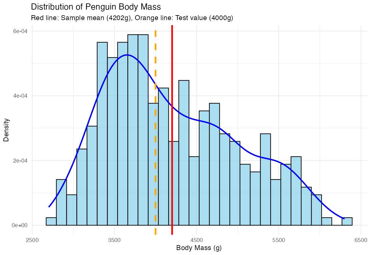
This plot shows the distribution of penguin body masses with both our sample mean (red solid line) and the test value of 4000g (orange dashed line). The clear separation between these lines visually confirms why our t-test found a significant difference.
Assumptions & Limitations
When NOT to use a one-sample t-test:
- Non-normal data with small samples: If your data is heavily skewed or has extreme outliers and n < 30, consider non-parametric alternatives like the Wilcoxon signed-rank test
- Dependent observations: If your data points aren’t independent (like repeated measures from the same subjects), use paired t-tests or mixed-effects models
- Multiple comparisons: Testing many hypotheses simultaneously inflates Type I error rates
What to do when assumptions are violated:
# Check normality with Shapiro-Wilk test (for small samples)
shapiro.test(body_mass[1:50])  # Only works for n ≤ 5000

# Visual normality check
ggplot(data.frame(body_mass), aes(sample = body_mass)) +
  geom_qq() + geom_qq_line() + theme_minimal()

# If normality is violated, use Wilcoxon test
wilcox.test(body_mass, mu = 4000, alternative = "two.sided")
Common Mistakes
1. Confusing one-sample with two-sample tests New users often use t.test(group1, group2) when they mean to test one group against a fixed value. Remember: one-sample compares to a number, two-sample compares two groups.
2. Ignoring the alternative hypothesis direction Always specify whether you expect the mean to be greater than, less than, or simply different from your test value:
# Two-sided (default): mean ≠ 4000
t.test(body_mass, mu = 4000, alternative = "two.sided")

# One-sided: mean > 4000
t.test(body_mass, mu = 4000, alternative = "greater")
3. Misinterpreting p-values A p-value of 0.03 doesn’t mean there’s a 3% chance your hypothesis is wrong. It means that if the null hypothesis were true, you’d see results this extreme or more extreme 3% of the time.