How to use geom_violin() in R
Introduction
The geom_violin() function from the ggplot2 package creates violin plots, which are a combination of box plots and kernel density plots. These plots show the distribution shape of continuous data across different categories by displaying the probability density of the data at different values. Violin plots are particularly useful when you want to compare distributions between groups while seeing both summary statistics and the full shape of the data distribution. They’re especially valuable when your data has multiple peaks, unusual distributions, or when you want to visualize the density of observations at different values. This function is part of the ggplot2 package, which is included in the tidyverse collection of packages.
Syntax
geom_violin(
  mapping = NULL,
  data = NULL,
  stat = "ydensity",
  position = "dodge",
  ...,
  draw_quantiles = NULL,
  trim = TRUE,
  scale = "area",
  na.rm = FALSE,
  orientation = NA,
  show.legend = NA,
  inherit.aes = TRUE
)
Key Arguments: - draw_quantiles: Numeric vector of quantiles to draw as horizontal lines - trim: If TRUE, trim the tails of violins to data range - scale: How to scale violins (“area”, “count”, or “width”) - position: Position adjustment (“dodge”, “identity”, etc.) - alpha: Transparency level (0-1) - fill: Fill color for violins - color: Border color for violins
Example 1: Basic Usage
library(tidyverse)
library(palmerpenguins)

# Basic violin plot
ggplot(penguins, aes(x = species, y = body_mass_g)) +
  geom_violin() +
  labs(title = "Distribution of Body Mass by Penguin Species",
       x = "Species",
       y = "Body Mass (g)")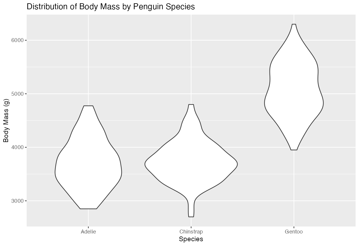
This creates a basic violin plot showing the distribution of penguin body mass for each species. Each violin shows the kernel density estimate of the data - wider sections indicate where more data points are concentrated, while narrower sections show fewer observations. The plot reveals that Gentoo penguins tend to be larger and have a different distribution shape compared to Adelie and Chinstrap penguins, which have more similar but still distinct distributions.
Example 2: Practical Application
# Enhanced violin plot with quantiles and styling
penguins |>
  filter(!is.na(body_mass_g)) |>
  ggplot(aes(x = species, y = body_mass_g, fill = species)) +
  geom_violin(draw_quantiles = c(0.25, 0.5, 0.75),
              alpha = 0.7,
              trim = FALSE) +
  scale_fill_manual(values = c("Adelie" = "#FF8C00",
                               "Chinstrap" = "#A034F0",
                               "Gentoo" = "#159090")) +
  theme_minimal() +
  theme(legend.position = "none") +
  labs(title = "Penguin Body Mass Distribution by Species",
       subtitle = "Violin plots with quartile lines",
       x = "Species",
       y = "Body Mass (g)",
       caption = "Data: Palmer Penguins")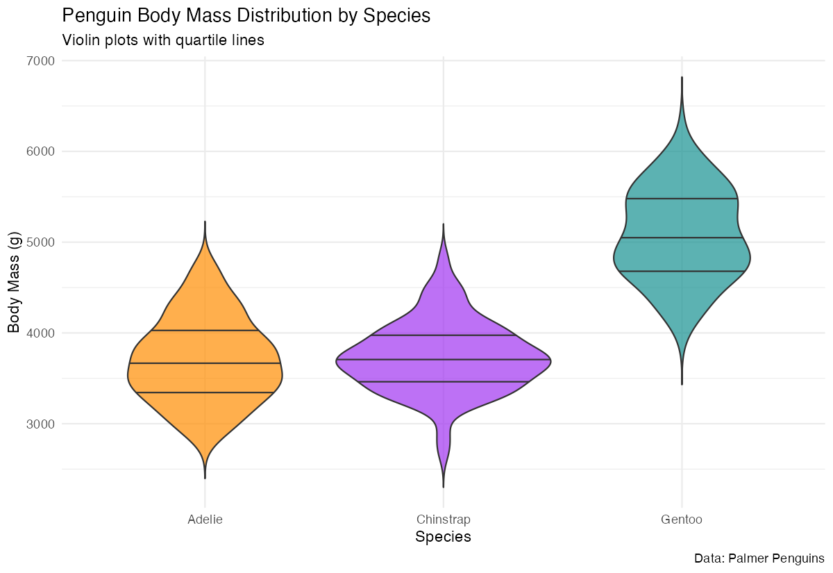
This enhanced example filters out missing values, adds quartile lines to show the 25th, 50th (median), and 75th percentiles, applies custom colors for each species, and uses better styling. The trim = FALSE argument shows the full kernel density estimate without cutting off the tails, and the transparency (alpha = 0.7) makes overlapping elements more visible.
Example 3: Advanced Usage
# Grouped violin plot with additional variables
penguins |>
  filter(!is.na(body_mass_g), !is.na(sex)) |>
  ggplot(aes(x = species, y = body_mass_g, fill = sex)) +
  geom_violin(position = position_dodge(width = 0.8),
              scale = "count",
              draw_quantiles = 0.5) +
  stat_summary(fun = mean, geom = "point",
               position = position_dodge(width = 0.8),
               size = 2, color = "white") +
  scale_fill_manual(values = c("female" = "#E69F00", "male" = "#56B4E9")) +
  facet_wrap(~island, ncol = 3) +
  theme_minimal() +
  labs(title = "Body Mass Distribution by Species, Sex, and Island",
       x = "Species", y = "Body Mass (g)", fill = "Sex")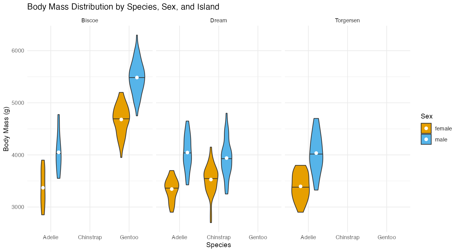
This advanced example demonstrates grouped violins by sex within each species, uses scale = "count" to make violin widths proportional to sample sizes, adds mean points with stat_summary(), and creates separate panels for each island using facet_wrap(). The position_dodge() ensures proper separation between male and female violins.
Common Mistakes
1. Forgetting to handle missing values:
# Wrong - may cause warnings or unexpected results
ggplot(penguins, aes(x = species, y = body_mass_g)) + geom_violin()

# Correct - filter or use na.rm
penguins |> filter(!is.na(body_mass_g)) |>
  ggplot(aes(x = species, y = body_mass_g)) + geom_violin()
2. Using inappropriate data types for aesthetics:
# Wrong - using continuous variable for x-axis grouping
ggplot(mtcars, aes(x = mpg, y = wt)) + geom_violin()

# Correct - use categorical variable or convert to factor
ggplot(mtcars, aes(x = factor(cyl), y = wt)) + geom_violin()
3. Misunderstanding the scale parameter:
# scale = "area" (default) makes all violins have same area
# scale = "count" makes area proportional to sample size
# scale = "width" makes all violins have same maximum width