How to use geom_density() in R
Introduction
The geom_density() function is a powerful visualization tool in ggplot2 that creates smooth density curves to display the distribution of continuous variables. It estimates the probability density function of your data using kernel density estimation, producing a smooth curve that shows where values are concentrated. This function is particularly useful when you want to visualize the shape, spread, and central tendency of your data distribution, compare distributions between groups, or identify potential outliers and multimodal patterns. Unlike histograms which can be sensitive to bin width choices, density plots provide a smooth representation that’s less dependent on arbitrary parameters. The function is part of the ggplot2 package, which is included in the tidyverse ecosystem.
Syntax
geom_density(
  mapping = NULL,
  data = NULL,
  stat = "density",
  position = "identity",
  ...,
  na.rm = FALSE,
  orientation = NA,
  show.legend = NA,
  inherit.aes = TRUE,
  outline.type = "upper"
)
Key Arguments: - mapping: Aesthetic mappings (usually x variable) - alpha: Transparency level (0-1) - fill: Fill color for the area under the curve - color: Color of the density line - adjust: Bandwidth adjustment (higher = smoother) - kernel: Smoothing kernel (“gaussian”, “epanechnikov”, etc.) - na.rm: Whether to remove missing values
Example 1: Basic Usage
library(tidyverse)
library(palmerpenguins)

# Basic density plot of penguin body mass
penguins |>
  filter(!is.na(body_mass_g)) |>
  ggplot(aes(x = body_mass_g)) +
  geom_density(fill = "steelblue", alpha = 0.5) +
  labs(title = "Distribution of Penguin Body Mass",
       x = "Body Mass (g)",
       y = "Density")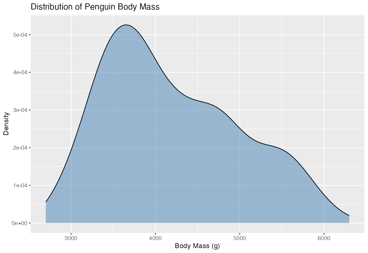
This creates a smooth density curve showing the distribution of penguin body masses. The curve peaks around 4000-4500g, indicating this is where most penguins’ masses are concentrated. The x-axis shows the actual body mass values, while the y-axis shows the density (probability per unit), not counts. The area under the entire curve equals 1, making it a proper probability density function.
Example 2: Practical Application
# Compare body mass distributions across penguin species
penguins |>
  filter(!is.na(body_mass_g)) |>
  ggplot(aes(x = body_mass_g, fill = species)) +
  geom_density(alpha = 0.7) +
  scale_fill_viridis_d() +
  labs(title = "Body Mass Distribution by Penguin Species",
       subtitle = "Gentoo penguins are notably larger than Adelie and Chinstrap",
       x = "Body Mass (g)",
       y = "Density",
       fill = "Species") +
  theme_minimal()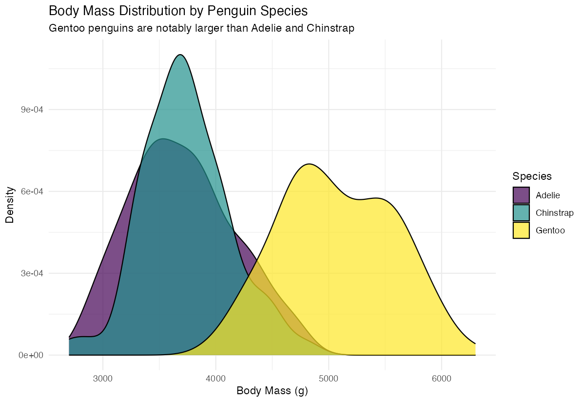
This practical example demonstrates how to compare distributions across groups. By mapping species to the fill aesthetic, we get separate colored density curves for each species. The alpha = 0.7 makes the curves semi-transparent so overlapping areas remain visible. This visualization clearly reveals that Gentoo penguins have a distinctly different (higher) body mass distribution compared to Adelie and Chinstrap penguins, which have similar distributions.
Example 3: Advanced Usage
# Advanced density plot with custom bandwidth and faceting
penguins |>
  filter(!is.na(body_mass_g), !is.na(sex)) |>
  ggplot(aes(x = body_mass_g, fill = sex)) +
  geom_density(alpha = 0.6, adjust = 1.5, color = "white", linewidth = 0.5) +
  facet_wrap(~species, scales = "free") +
  scale_fill_manual(values = c("female" = "#E69F00", "male" = "#56B4E9")) +
  labs(title = "Body Mass Distribution by Species and Sex",
       x = "Body Mass (g)",
       y = "Density") +
  theme_minimal() +
  theme(strip.text = element_text(face = "bold"))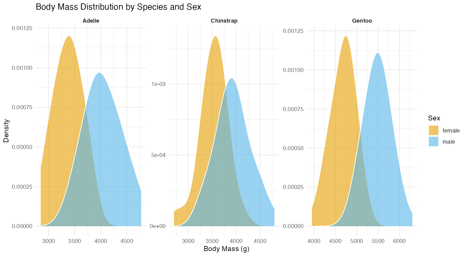
This advanced example combines density plots with faceting to show distributions by both species and sex. The adjust = 1.5 parameter creates smoother curves by increasing the bandwidth. Using facet_wrap() with scales = "free" allows each panel to have its own scale, making it easier to see patterns within each species. This reveals sexual dimorphism in body mass across all three penguin species.
Common Mistakes
1. Forgetting to handle missing values:
# Wrong - may produce warnings or unexpected results
ggplot(penguins, aes(x = body_mass_g)) + geom_density()

# Right - explicitly handle NAs
ggplot(penguins, aes(x = body_mass_g)) +
  geom_density(na.rm = TRUE)
2. Using density plots with discrete variables:
# Wrong - density plots are for continuous variables
ggplot(penguins, aes(x = species)) + geom_density()

# Right - use bar plots for categorical data
ggplot(penguins, aes(x = species)) + geom_bar()
3. Misinterpreting the y-axis as counts: Remember that density plots show probability density, not counts. The y-axis values represent probability per unit of x, and the total area under the curve equals 1. If you need counts, consider geom_histogram() instead.